Using Obsidian Bases for Car Shopping
Introduction
In my recent article, I explained some of the takeaways from my experience buying my first car. During the shopping process, I made extensive use of the note-taking app Obsidian. In particular, I used a recently added feature called Bases, which aggregates and displays information about your notes.
This feature is incredibly useful for collecting, organizing, and analyzing information. It worked well as I tracked candidates during the car-buying process, but it has many uses across a wide variety of contexts. If Obsidian had been around when I was a student, I’m sure I would have loved using it to manage my notes. Today, I use it for many things both at home and at work. At home, I use it for tracking my exercise routine, for shopping comparisons, and for other things like reading lists. The Obsidian Bases roadmap also mentions a Kanban mode, which I’m currently using other plugins for.
In this article, I describe how I set up my Base to power my car-shopping process. I show how to create a Base, filter it, create custom formulas based on note properties, group items, and create custom views to display your data in different ways. To do that, I’ll explain each feature as I used it in my car-buying context.
How Obsidian Bases work
A Base displays metadata about the notes in your vault (Obsidian-speak for all your notes). When you first create a Base, it shows a table that lists every note in the vault. The Base provides an easy way to:
- filter the list of notes, both globally and per view,
- show, hide, and add metadata to your notes,
- create new notes for the Base, and
- customize how the data is displayed through custom views and grouping.
All of these things can be changed via the buttons in the header of the Base, shown below.
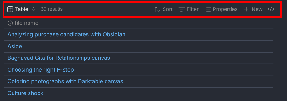
You can do almost all of your configuration with these options at the top of the table.
Setting up a Base
In Obsidian, you create a Base either in a new file by using the file extension .base or by creating a code block with the base language code, like so:
```base
```
By default, an Obsidian Base lists every file in your vault. To limit what gets listed, choose a set of criteria based on file metadata. For my vehicle shopping, I set it to any file that had the #vehicle tag on it and that wasn’t located in the “Templates” folder.
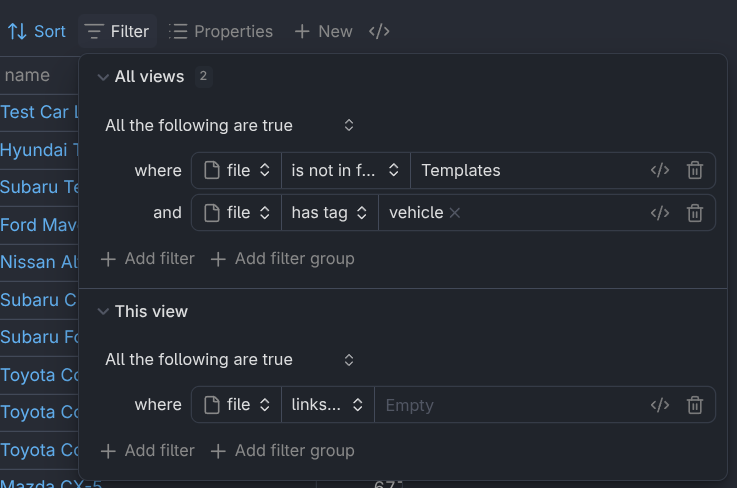
Set your main filters in the “All views” section, then use the bottom section to change filters for each view you create.
Then, I added several properties that would help me with the shopping process. If a note property doesn’t exist, you can type the name of a new one and press enter to create it. Each note you create with the “New” button will have those properties.
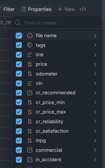
Create or add properties to the view via this menu.
One of the nice things about Obsidian Bases is that you can add and edit entries right inside the table. It’s a great feature, although you have to press enter on each field that you want to edit (except for checkboxes). Obsidian Bases are still under active development, so I expect this will improve over time.
Data collection
With the Base set up, I started creating entries for each car to consider. I covered this process in my previous article, but below is a summary of the properties I filled in for each listing:
- The title and URL of the listing: the title of the listing became the name of the note
- The mileage, VIN, and asking price.
On Consumer Reports, I searched for the make, model, and year. Then, I noted the following information:
- The reliability and owner satisfaction scores
- The market price minimum and maximum
- The fuel economy: I defaulted to the in-city number since most of my driving would be between home and work
Finally, for cars I was more interested in, I also looked at the vehicle history report from CARFAX or similar services, if it was available on the car listing. Often, I would only collect this information after having looked at several candidates. Having a link to the listing made it easy to go back for more information. On the history report, I noted the following information:
- Whether the vehicle was used commercially
- If any accidents had been reported
In total, I collected seven pieces of information for each vehicle. These data points form the foundation to use one of the Base’s most useful features: formulas.
Creating metrics to compare vehicles
In addition to note properties, Obsidian Bases also lets you use formulas to perform more advanced analysis. I created several of them, which I detail below.
First, since the year, make, and model were all in the file name, I created some simple formulas to show them in their own columns in the Bases table. This made it possible to sort the candidates more easily.
Formulas are easy to create, though much like Excel formulas, you do have to have a basic understanding of functions and data types, like what strings, numbers, and lists are. While that’s outside the scope of this article, the examples below, the official documentation, and maybe some conversations with an LLM will get you started making your own formulas.
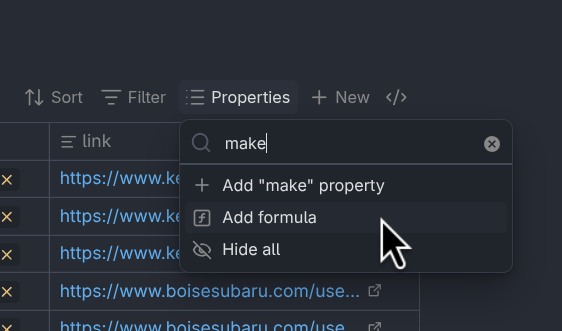
Click “Add formula” to create a new formula, then enter the formula in the box.
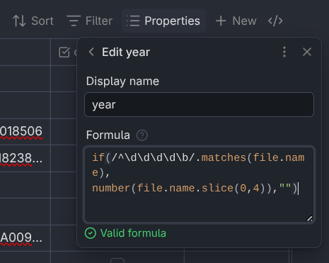
Extracting the year, make, and model from the file name
The model year of each car was always the first word in the note name, so I used the following formula to extract it: if(/^\d\d\d\d\b/.matches(file.name), number(file.name.slice(0,4)), ""). This uses the if() function, which works a lot like the function of the same name in Excel. First, give a condition, then the value if true, and last, the value if false. Each parameter is separated by a comma.
To help explain how the formulas work, let’s take an example note with the name “2019 Honda CR-V EX-L AWD.”
The formula that extracts the year from the file name demonstrates how you can use regular expressions (practice them here) to match strings of text. In this formula, /^\d\d\d\d\b/.matches(file.name) checks to see if the file name starts with four digits and a word boundary (\b). If it matches, then the formula number(file.name.slice(0,4)) gets the first four characters of the file name and converts them to a number. If the file name doesn’t match the regular expression, then it returns nothing (""). Altogether, this extract the 2019 from our example note’s name.
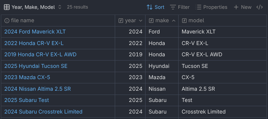
For the car’s make and model, I used the split() function to break the file name into pieces separated by spaces. This function returns a list of strings that you can use square bracket syntax to select from, like this: file.name.split(" ")[1]. The list starts at zero, so [1] means to get the second item in the list. The car’s make is almost always the second word in the note name, so in our example, this function would return Honda.
To get the model, I decided it would be simplest to just get everything after the first two words in the file name. To do that, I used the powerful filter() function. The formula file.name.split(" ").filter(index > 1) uses the filter function’s built-in variable index to check each word’s position in the list. If it comes after the second word (index > 1), then keep it. Given the example note name, this would show CR-V EX-L AWD.
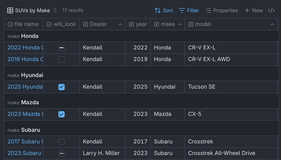
With these three filters in place, I could now sort by each of them as I wanted by simply clicking the column name. In the example below, I’ve sorted first by make, then by model year, most recent year first.
You can use calculated formula columns to sort.
Comparing the asking price to market rates
Next, I wanted to see at a glance whether the car’s asking price fell within the market price range that CR suggested. This formula may look a little intimidating, but it is really just a chain of yes-no questions.
if(
 price.isEmpty() || cr_price_min.isEmpty() || cr_price_max.isEmpty(),
 "unknown",
 if(
   price < cr_price_min,
   "undervalued",
   if(
     price <= cr_price_max,
     "typical",
     "overvalued"
   )
 )
)
This formula returns four possible values, checking each of them in order:
unknownif one of the required price-related properties is missing,undervaluedif the asking price is below the CR price minimum,typicalif the asking price is inside the CR price range, andovervaluedif it’s above the high end.
This “decision tree” of sorts is accomplished with nested if() functions. This will seem very familiar to long-time Excel users. Bases formulas allow you to check if a property is empty using the isEmpty() function. You can also string together several conditions using the double pipe operator ||.
Parse the dealer location from the URL
I used the contains() string function to show which dealer the car was at with the following string of if() statements. It just looks at the URL to the car listing on the dealer’s website and checks for known web domains. This formula became incredibly useful when I was ready to actually go out and shop. With Bases, you can group rows together by any property, so I used this field to help plan my itinerary on shopping days. (I show how this works in a later section.)
if(link.contains("kendall"), "Kendall",
if(link.contains("mhauto"), "MH Auto Ranch",
if(link.contains("peterson"), "Peterson",
if(link.contains("boisesubaru"), "Larry H. Miller",
if(link.contains("carmax"), "CarMax",
if(link.contains("tvsubaru"), "Treasure Valley Subaru", "Unknown"
))))))
Expected mileage
I used the following formula to calculate the average expected mileage for a car given its model year:
((file.ctime - date((formula.year - 1) + "-10-01")).days * (13756/365)).round()
The formula has several parts. First, I created a date to start accumulating the miles with date((formula.year - 1) + "-10-01")). This assumes that the car was sold on October 1st of the year prior to the model year, since most model years tend to come out in fall of the previous year. Then, I subtract the result from file.ctime, which is when the note was created. This formula assumes that the car was driven up until the day I found its listing, which isn’t accurate, but it keeps the formula relatively simple. Adding .days to the end of that gives the number of days between the two dates.
Then, I multiplied that by the average number of miles driven per day in Idaho, where I live. A Google search led me to 13,756 miles per year divided by 365, or about 38 miles per day. This number tells me how many miles each car would have if its previous owners drove the average number of miles every day. The number is a back-of-napkin estimate that hints at how a given car was used, when combined with other information about the car.
Adjusted life expectancy
Based on my cursory research, most SUVs and sedans from large automakers can expect a total of around 200,000 miles over the life of the vehicle. Using this as a baseline, I created an adjusted mileage life expectancy in terms of each vehicle’s CR reliability score, .
This is called a piecewise linear regression model, where is the reliability score for the car, is the baseline life expectancy for all vehicles, and each is a mileage factor that scales the life expectancy. When charted, the formula has the angled shape shown in the graph below.
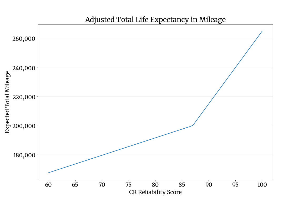
The hinge in the line is at the average reliability score for my candidate pool, 87.
The average reliability score in my candidate pool was 87, with a few cars reaching as low as 66, and several cars (mostly sedans from Korean and Japanese automakers) with scores in the 90s. I adjusted each until they approximated the range of mileage I could expect based on my research. I used this function instead of a standard linear regression because of how high the average reliability score was—a single line couldn’t accommodate both the lower and higher end of the range of reliability scores.
To help ensure formula legibility, it helps to break the complex formulas into smaller formulas and use them together in the end result. To that end, I created the following helper formulas.
| Bases formula | Value / Formula | Description |
|---|---|---|
life | 200000 | Baseline lifetime mileage |
avg_rel | 87 | Average reliability score |
life_rel_bonus | 5000 * max(0, cr_reliability - formula.avg_rel) | Reliability bonus (beta–max term) |
life_rel_penalty | 1200 * min(0, cr_reliability - formula.avg_rel) | Reliability penalty (beta–min term) |
The final formula uses these terms like this: (formula.life + formula.life_rel_bonus + formula.life_rel_penalty) * if(commercial, 0.9, 1). The last if() statement further reduces the score by ten percent if the car had a history of commercial usage.
Estimating overall value for money
One of the reasons I developed the metric was to be used in a calculation of price per remaining mile (PRM). In other words, I wanted to estimate how much each mile would cost me in the long run. Adjusting the expected lifetime mileage of the car served as a proxy for other factors, such as fuel, repair, and insurance costs over the lifetime of the vehicle. Without it, I would have to do a lot more research and create a much more complex formula than this one. In this case, simplicity and convenience were more valuable than rigorous accuracy.
The formula (price/(formula["L(R)"] - odometer)).round(2) returns the price per remaining mile metric. This shows the dollar value of the car in terms of the cost of each mile I can expect to get out of the vehicle. The odometer property is the mileage of the car. Most cars I looked at fell between $0.14 and $0.18 per mile, with the lowest being $0.11 and the highest being $0.57. Multiplying that by the average number of miles driven in a year, that adds up to a difference of more than $6,000 per mile-year.
Creating views to display the data in different ways
Having created Bases formulas for the metrics I was interested in, I created different views to present the data in different ways. See the official documentation for views here.
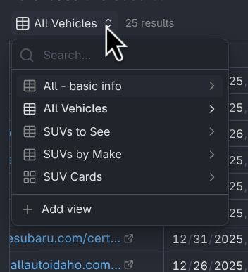
Select or add new views with this menu.
Each view can have its own set of filters, ordering, grouping, and layout. The image above shows a few examples of views I created during my car search.
Using the grouping feature, you can group your notes into different categories.
Note that when you’ve created multiple views, you can choose one to be the default view when you open the file.
Grouping
One feature I used extensively was the grouping feature. This feature allows you to put each item into a group based on a property. You can even group by properties not shown in the view by showing the column, grouping by it, then hiding it again.
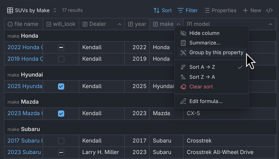
To group by a property, right-click the header and click the “Group by this property” option.
When I was ready to narrow down my list of vehicles to a few finalists, I added a will_look checkbox property to the Base, then checked the box for each one I wanted to look at. I then made a view that showed only those vehicles, grouped by dealer so I could plan out which dealers to go to and in which order.
Final thoughts
There are other features of Obsidian Bases I haven’t covered in this article. Not only can you show results in tabular format, but you can also create cards with images, lists, and even maps to display your data. It’s a really powerful tool.
The only thing I feel needs improvement is the data entry process. It’s not too bad as it is, but having to hit enter to edit each field in the table can be a little tiresome after a while. This would be one reason why one might choose to use another tool such as Excel. For me, however, the portability, modern built-in functions and data types, and the ability to quickly create custom views for the data make it a winning choice.