Machine Learning Approaches to Marketing in the Banking Sector
Contents
Yi, et al. (2020) noted that data collected by organizations often goes unused in creating customer value. Businesses may lack the resources or expertise to take advantage of the data collected. This reveals an opportunity for businesses to implement machine learning (ML) to process, aggregate, and analyze data. To explore this opportunity, I evaluate a set of six common ML models to determine which most effectively predicts subscription outcomes in a marketing campaign.
The dataset comes from a Portuguese financial institution’s direct marketing campaign for term deposits. It’s publicly available from the UC Irvine Machine Learning Repository. The goal is to predict whether a given customer will subscribe to a term deposit based on the business and personal information available about the client.
The dataset consists of about 45,000 samples of previous client interactions, each labeled according to whether the client subscribed to the product. Its 20 input variables include factors like age, marital status, when the client was last contacted for a campaign, and economic indicators such as the monthly consumer confidence index.
This project illustrates how machine learning can be used to support data-driven decisions in a business context. It’s structured in three parts: methods, results, and discussion. First, in the methods section, I describe the data cleaning process and perform an exploratory analysis of the data (EDA). Then, I describe the ML model selection and training process. Finally, I describe the results of the prediction task and discuss some limitations and implications.
Methods
Data cleaning and exploratory analysis
The first step in the data analysis process is to import and clean the data. The published version of this dataset has no missing values, saving some time in the cleaning process.
In this dataset, only about thirteen percent of samples indicate a successful outcome, where the client subscribed to the product. This indicates a strong class imbalance, where one class (“no, the client didn’t subscribe”) has many more samples than the other class (“yes, the client subscribed”). This has implications for the interpretation of accuracy metrics, which I’ll discuss in the results section.
Importantly, I removed one feature from the set of input variables. Call duration isn’t applicable to the prediction task because the marketing agent would know after the end of the call whether the call was successful or not. So, using the length of the call only provides a post hoc indication of success.
Exploratory analysis revealed some interesting correlation patterns between data points. The heatmap below shows correlation values between the variables in the dataset. Lighter and darker colors indicate stronger positive and negative correlation between variables, while magenta indicates weaker correlations. Client age appears not to correlate strongly with any variable. Positive outcomes (y_yes in the heatmap) show moderate inverse correlation with two socioeconomic indicators: average number of employed citizens (nr.employed) and the Euribor 3-month rate (euribor3m). It also appears that the number of days since the client was last contacted is a significant factor at -0.32. Previous successful outcomes (poutcome_success) are also correlated with positive outcomes at 0.32.
While some variables correlate with positive outcomes, no single variable stands out as a strong predictor of campaign success. The model evaluation phase provides an opportunity to confirm what significant factors contribute to successful predictions.
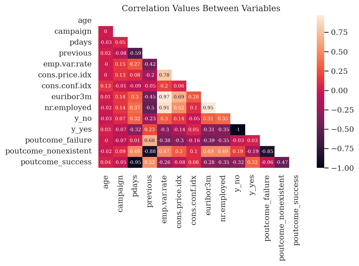
Lighter colors indicate stronger positive correlations. Darker colors indicate stronger negative correlations. Magenta represents weaker correlations.
Model selection
To predict outcomes, I selected six common ML models as candidates for testing. I selected the -Nearest-Neighbors (KNN), Linear SVM, standardd SVM, and Logistic Regression (LR) classifiers. I also included a Random Forest (RF) classifier and an MLP classifier, which is a popular type of neural network. The first four models are distance-based models, meaning they work by calculating the distance between points in the data. RF is a tree-based method, meaning it creates a group of randomly chosen decision trees and averages them together to make predictions. RF is one of the most common non-distance-based classifiers.
I selected these models for their popularity and to demonstrate the performance of a variety of model types. KNN is typically one of the fastest models available, though not always the best performer. The SVM models are powerful but resource-intensive, while LR strikes a balance between the two. Lastly, I included MLP because the authors of the introductory paper for this dataset found it to be the best performer, and I wanted to compare my results with theirs.
Data preparation
For each model, I created a processing pipeline that scaled the data and one-hot encoded it. Scaling and one-hot encoding were applied as part of the pipeline for distance-based models, while the other models used just one-hot encoding.
Data scaling involves adjusting the values so that the mean centers on zero and the standard deviation equals one. This rescaling of the data can greatly improve the performance of distance-based models.
While scaling applies to continuous variables, one-hot encoding splits categorical variables with multiple values as separate binary variables. For example, in this dataset, the variable education could have the values university.degree, high.school, unknown, and so on. One-hot encoding creates variables like education_university.degree and assigns it a value of true or false. This is required by most models in the Python library used to train the models. (I used Scikit-Learn, which has a comprehensive set of ML models with a uniform API.)
In order to cross-validate the results, I split the dataset into three parts: a training set, a validation set, and a final “holdout” set. The first two sets formed a training-validation loop, where the training set was used to train each model and the validation set provided a means for verifying the results of each iteration. The holdout set was used only after the model training process was complete. I tested each model on the holdout set at the end of the process to provide an example of model performance on truly unfamiliar data.
Model parameter selection and training
To tune each model, I tested a variety of parameters for each model to identify the best-performing configuration.
I selected the following metrics to assess model performance during the training process. First, the receiver operating characteristic (ROC) area under the curve (AUC) provided an overview of how well the model predicted successful cases versus false positives. Second, the balanced accuracy score showed the mean accuracy of positive and negative predictions. This score was chosen to mitigate the problem of class imbalance, where too few of the positive or negative cases can skew results. I discuss the choice of metrics more in the limitations section below.
In a classification task like this one, ML models choose either a “yes” or a “no” with a decision function. This function varies by model, but the models work by processing the data for each sample, returning a single number for each one. It then compares that number to a threshold. If the number is higher than the threshold, it gets one class; if it’s lower, it gets the other. For probabilistic models like RF, the default threshold is 0.5 (between the minimum of zero and the maximum of one). For others the default threshold is often zero.
Often, the default threshold doesn’t yield the best results. The model can be tuned to find the best threshold for maximizing a given metric. In this project, I tuned each model to maximize the balanced accuracy score. I chose balanced accuracy to compensate for a significant class imbalance, mitigating the risk of a misleading accuracy score.
Results
Model performance
The majority of machine learning models gave similar performances. One exception was the SVM classifier, which proved impractical to train because of system restraints. I assessed overall performance using the area under the curve (AUC) of the receiver operating characteristic (ROC) graph, which shows how well the model did at predicting the target customers while avoiding false positives. Generally speaking, the larger the AUC, the better the model’s predictions were.
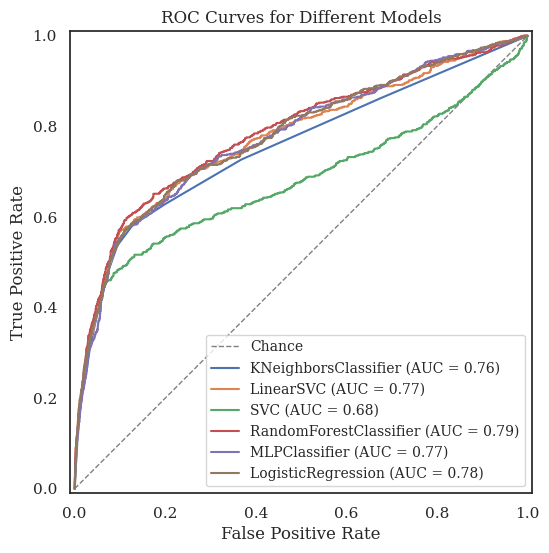
Most models tested performed well above the baseline of chance. The RF classifier had the best performance of the group, though only marginally. By comparison, the Linear SVC model achieved similar results, but required only half the training time.
In second and third place, by a small margin, were the LR and MLP classifiers. LR was also the second fastest in training, slower only than the -Neighbors classifier and nearly three times as fast as RF. In a resource-limited context, Linear SVC or LR would be good choices to balance performance and resource usage.
Meanwhile, MLP took 2.7 seconds to train, about four times as long as RF. Its AUC of 0.775 earned it a close third place behind LR. In the study which published this dataset, the authors reported an MLP as having the best performance. Due to resource constraints and dataset differences, I was unable to replicate their result. However, the scores from my results are similar to each other, so the ranking difference could be attributed to chance. Read their original paper here.
| Model | Training time | AUC | Bal. accuracy | Decision threshold |
|---|---|---|---|---|
| SVC | 8.049 | 0.677 | 0.676 | -0.957 |
| MLPClassifier | 2.661 | 0.775 | 0.726 | 0.030 |
| KNeighborsClassifier | 0.095 | 0.756 | 0.727 | 0.162 |
| LogisticRegression | 0.285 | 0.777 | 0.728 | 0.153 |
| LinearSVC | 0.344 | 0.774 | 0.730 | -0.699 |
| RandomForestClassifier | 0.678 | 0.785 | 0.740 | 0.145 |
The standard SVC took much longer than other models to train, but performed the worst out of the group with an AUC of 0.677, fifteen percent lower than RF. The SVC model was extremely resource intensive, making it impractical to do a comprehensive search for optimal model parameters. Because of this, I trained the model using its default parameters. I have included its results mainly for reference, as it shows that not all models are equally suited to a particular task.
Interpretability of model predictions
During the EDA phase, I identified several variables which would be possible predictors of successful campaign outcomes. Analysis of feature importance from each model mostly confirms the initial analysis.
To reveal which input variables contributed the most to a model’s predictions, I used permutation importance, which scrambles each input variable one at a time while tracking the relative effect on performance. This technique answers the question, “How would my performance be affected if I didn’t have this variable?” For each model, economic indicators took the top two spots for importance, reflecting what the correlation matrix revealed. Personal factors varied more in importance. Below are the top ten features reported for RF.
| Rank | Feature | Mean importance | Std. importance |
|---|---|---|---|
| 1 | Euribor 3-month | 0.027890 | 0.014443 |
| 2 | Employment variance rate | 0.025940 | 0.012559 |
| 3 | Avg. # of employed citizens | 0.014691 | 0.009048 |
| 4 | # of contacts for current campaign | 0.005932 | 0.006990 |
| 5 | Age | 0.005234 | 0.006940 |
| 6 | Job | 0.003863 | 0.007745 |
| 7 | Education level | 0.003499 | 0.008755 |
| 8 | Month of last contact | 0.003124 | 0.008162 |
| 9 | Days since previous contact | 0.001516 | 0.002469 |
| 10 | Has housing loan | 0.001363 | 0.006586 |
The number of contacts made with the client during the current campaign contributes to successful prediction of outcomes. More information about the content of previous calls would help further improve this variable’s predictive power, but this is a limitation of the current data set. Surprisingly, client age is a relatively important predictor of successful campaign outcomes, considering its limited correlation with other variables. Behind that, features that contribute to successful outcomes include client occupation, education level, temporal information about the last contact with the client, and whether the client has a housing loan.
Results validation
The final results I’m publishing here are based on data that each model had never seen before. Using unseen “holdout” data for testing helps ensure the model didn’t over-fit to the training data. Using cross-validation during the training process also helped prevent over-fitting. AUC and balanced accuracy scores from the holdout test correspond closely values seen during the testing phase, varying no more than five percent. This indicates a well-trained model.
Limitations
Several limitations should be considered when evaluating the results of this test. The first consideration is performance. The neural-network-based MLP classifier is well known to be difficult to tune. A more comprehensive grid search may yield better results than what I was able to accomplish with project resources.
Limited resources also contributed to the poor performance of SVC. Possible solutions include reducing the number of features using principal component analysis before training, or training on a subset of the data.
A second limitation of this project is the choice of metric for assessing model performance. This project used the balanced accuracy score, which averages sensitivity and specificity to help mitigate the effects of class imbalance (i.e. having many more “didn’t subscribe” than “subscribed” samples in the dataset). However, balanced accuracy gives equal weight to false positives and negatives, which may not fit the business case. In this project, a false positive means marketing to a customer who is not likely to subscribe to the product, while a false negative means missing an opportunity to market to a customer who is likely to subscribe.
One possible solution is to write a custom cost function that weights each outcome based on business logic. For example, the marketing manager might determine that missed opportunities are 1.5 times as costly as false positives. The custom cost function would then be able to choose a threshold that gives the best result based on this criterion. Scikit-Learn’s documentation has an excellent example of this process.
Discussion and conclusion
The results of this project have demonstrated the viability of machine learning as a tool for predicting the outcomes of direct marketing efforts in a banking context. The majority of models tested showed balanced accuracy scores of nearly 0.75, indicating an outcome prediction probability much higher than chance.
The results have significant implications for a business manager. For example, if the direct marketing manager needed to cut costs by reducing the total number of direct marketing calls made by the department, a machine learning model could suggest a list of clients with the best chance of success. This provides the manager with evidence-based, data-driven support for important business decisions.
To conclude, this project evaluated the performance of several popular ML models for predicting direct marketing outcomes at a financial institution. The results demonstrate how ML can be used to support evidence-based, data-driven business decisions. Future work with this dataset could include the development of a cost-sensitive model to better reflect real-life trade-offs and organizational priorities.